![]()
 SWAG: Software
Architecture Group
Using the CLICS clone detector and GUI
For the most recently available documentation dowload the external pdf documentation or go to the CLICS wikki.
Synopsis
This document will describe how to detect and analyze code clones in a software system using the CLICS clone detector and GUI. This process is broken into 4 steps:
1) Environment setup.
2) Clone detection.
3) Postprocess code clones (filter and categorize).
4) Investigate and annotate code clones using user interface.
Note, throughout this document, shell commands will be provided as examples. Each command will begin with `$>' indicating the shell prompt.
This is an initial draft of a help document. It does not yet contain documentation of all of the options for the commands used here.
Step 1: Environment Setup
Part of the clone detection process is the extraction of code regions from within C/C++ source code. These code regions include procedure bodies, macros, and data type definition such as unions and structs. CLICS uses a modified version of ctags to do this and uses the environment variable CTAGS_PATH to find the executable. Before running the clone detection, postprocessing, or UI steps be sure to set the path to the modified ctags executable. For example, in bash you would export the variable with the following command (assuming ctags-mod can be found in /usr/local/bin):
$> export CTAGS_PATH=/usr/local/bin/ctags-mod
Step 2: Clone Detection
Clone detection is comprised of three steps: building a list of source files, source code region extraction, and running the clone detector. In the first step, we must construct a file containing a list of source files, one per line. The files should be listed using their full path, not their relative path. This can be conveniently done using find (newer versions of find support more advanced regex operators than the example given here):
$> find /home4/cjkapser/Research/cases/pine -name “*.c*” >> pinefiles
$> find /home4/cjkapser/Research/cases/pine -name “*.h*” >> pinefiles
This file will now contain a list of the source files used to build pine. Note in the above example the full path to the source directory is given as the path argument for find.
Next we must extract the regions (procedures, macros, etc.) from the source code. This is done using the command `ExtractRegions.py'. In its typical usage ExtractRegions.py requires two options to be specified: -o output_file and -f input_filelist. -o specifies the output file that will contain the extracted regions, -f specifies the location of the list of files to extract regions from. Ex: $> ExtractRegions.py -f pine-files -o pine-regions
Todo: document region file format.
Once this list of regions is extracted, we can start the clone detection:
$> clics_clone_detection -M 2304 -m 60 -o pine-clones -R pine-regions
This command takes several options. -M defines the approximate memory to be used to store the suffix tree data structure (the core data structure for locating the code clones). With 4GB total RAM, 3 GB of available RAM on a 32 bit OS, it is generally safe to use 2.25 GB for the suffix tree, leaving ample room for opening files and search for clones. -m specifies the minimum number of lexical tokens that must compose a match for it to be valid. The default is 30 tokens, the above example specifies a minimum of 60 tokens. -o specifies where to place the output of the clone detection process, the above example places the clone output in pine-clones. -R specifies the input file where the extracted regions from the previous step can be found. The complete option summary of clics_clone_detection is:
| -p | Parameterize the input (replace identifiers with placeholder and force a semi one-to-one match to filter matches). [conflicts with e and r] |
| -r | Use raw input, do not tokenize or parameterize. [conflicts with e and p] |
| -e | Use tokenized input, do not parameterize. [conflicts with p and r] |
| -M | Amount of memory to use for suffix tree. |
| -m | Minimum size (in tokens) for an acceptable clone. |
| -o | Output file [must be specified]. |
| -R | Region file to use to split clones into regions (rather than allow them to cross multiple regions. If not specified, command expects a file containing a list of source files as an argument. |
Todo: document clone file contents.
Step 3: Postprocessing code clones (filter and categorize)
Once the code clones are detected they need to be filtered, categorized, and loaded into a postgresql database. Ex:
$> ConvertToPostgres.py -d pine_clones_60 -f pine-clones
This command will create a database `pine_clones_60' and filter it with filtered and classified clones from the set of clones found in the file `pineclones'. The option -d specifies the database to create, -f specifies the input file. The complete list of options taken by this command are:
[-h host -p port] [-u username] [-P] -d dbname -f filename
| -h | hostname of database server |
| -p | port number the postgresql server is listening on |
| -u | username to connect to database with |
| -P | ask for a password before connecting |
| -d | database name to create |
| -f | file containing clones to be filtered and loaded into the database |
Todo: document the 6 filters, the categorization, and the database relations.
Summary of Steps 1, 2, and 3
$> #Set up environment
$> export CTAGS_PATH=/usr/local/bin/ctags-mod
$> # Make a list of files to detect clones $> find /home4/cjkapser/Research/cases/pine -name “*.c*” >> pine-files $> find /home4/cjkapser/Research/cases/pine -name “*.h*” >> pine-files
$> # Extract the region information from the files
$> ExtractRegions.py -f pinefiles -o pine-regions
$> # Detect clones using region information
$> clics_clone_detection -M 2304 -m 60 -o pine-clones -R pine-regions
$> # Post process clones and load them into a database
$> ConvertToPostgres.py -d pine_clones_60 -f pine-clones
Step 4: Investigate and annotate code clones using user interface
Analyzing clones in software involves inspecting individual clones to manually filter false positives and annotate valid clones. Both of these tasks are highly subjective, and the quality of the process depends very strongly on an understanding of the software being analyzed. It is strongly recommended that design documentation is reviewed and, if necessary, investigate/document the important data structures and subsytems before beginning this step. The goal of this software review is to gain an understanding the software system similar to that which you would need to maintain/enhance the software because the decisions you make about code clones should be considered in this context.
Once you have an understanding of the software system, you can open the CLICS user interface with the following command:
$> CLICS_GUI.py
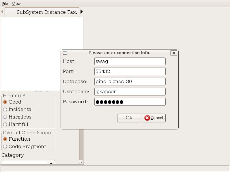
Open the code clone database you created earlier (during postprocessing) using the File → Open DB menu item. You are presented with a dialog (Figure 1). All fields are optional with the exception of Database. Host is the name of the server hosting the postgresql database, port is the port postgresql is listening on, database is the name of the database containing the clones, username and password are the authentication credentials used to connect to the database. If you are running CLICS on the same machine as the host database, you can often just input the database name.
In order to browse the code clones, you must have the source code of the software system on your local filesystem. If you are browsing the code clones on a different machine from the one where the code clone detection was performed, you may need to adjust the prefix of the file locations. This can be done using the menu item File→ Change Source Dir (Figure 2). The text shown in original path will be replaced by the text in new path. For example, if the path the source files during detection was “/home4/cjkapser/Research/cases/pine/...” and the source location on the machine running CLICS_GUI is “/home/cjkapser/Research/cases/pine” we can replace the beginning of the path with the information shown in Figure 2. This step is required each time you connect to a clone database.
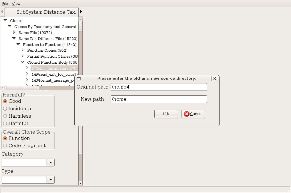
Figure 2: Change Source Directory Prefix The anatomy of the user interface
The user interface of CLICS provides several views of clones and variety of forms of querying to select or find clones of interest. On the left hand side of the UI you will find tabs allowing you to browse clones by: a simple taxonomy (SubSystem Distance Tax. tab), filesystem (Files tab), query results organized by taxonomy (Query tab), a randomly selected clone (Random tab), and by annotated clones (Annotated tab). The rest of this section will discuss each of these tabs and the views of cloning they provide. You will also notice on the bottom left a form that can be used to document selected clones. You will see how to use this in the text that follows. The right hand side of the user interface changes depending on the tab left tab you have currently selected.
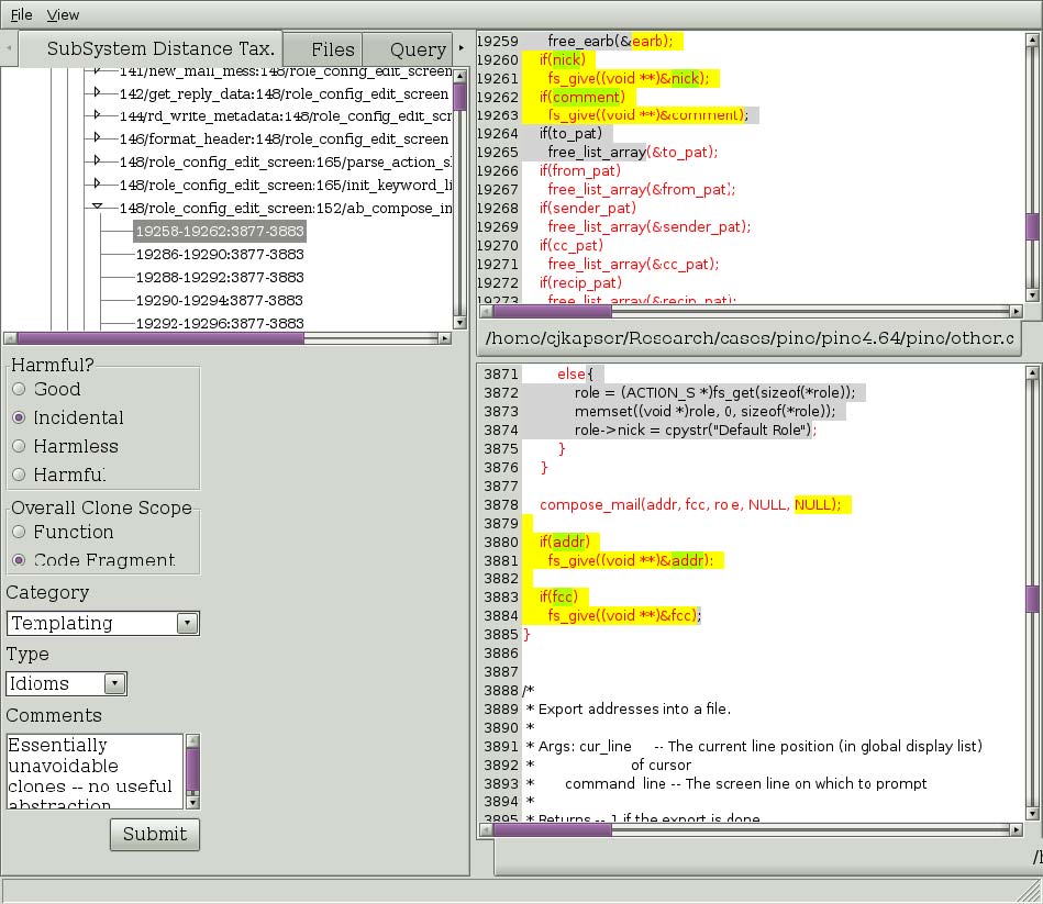
Figure 3: A clone selection in the subsystem distance taxonomy.
The default tab is the Subsystem distance taxonomy tab. This tab allows you to browse clones according to an automatic classification, described in [1]. The current implementation is not complete (in the middle of refactoring). See the tool for current level of implementation. To navigate clones in this tree select nodes in the tree. Each node represents a level in the taxonomy, indicated by the name of the node in the tree, until you reach a set of nodes labeled with the format “integer/string:integer/string” (ex. 148/role_config:152/ab_compose). This indicates you have hit the end of the categorization for this subtree, and the children are now Regional Group of Clones (RGCs). This is a set of clones that comprise the cloning between two regions. In Figure 3, on the left we see a RGC that has been expanded and one of the clones has been selected. On the lower left you can that the type of cloning this RGC contains has been filled in. The basis for the categories, harmfulness, and scope is documented in [2]. To commit annotations to the database, simply fill them in and select “Submit”.
On the right, the selected region is show in red text, and the selected clone is shown in yellow and green highlights. The highlighting provides an indication of overall clone similarity by illustrating the simple diff of the tokens of the two clones. Yellow highlighting indicates the tokens in the clones are the same, green indicates the tokens are different. This highlighting can be applied to the entire region if you wish to see the longest common subsequence between the regions. Simply right click on the TEXT of one of the regions and select “Diff regions” from the menu that will popup. You will also notice in Figure 3 that some of the text is highlighted in gray with black text. This indicates there are clones between the two files that are not part of this RGC. This is intended to provide information about the degree of cloning between the two files: scrolling through the two files will show more highlighted text. The reader should also node that each level of the tree is annotated by an integer “(integer)”. This integer indicates the number of clones contained in the subtree of each node.
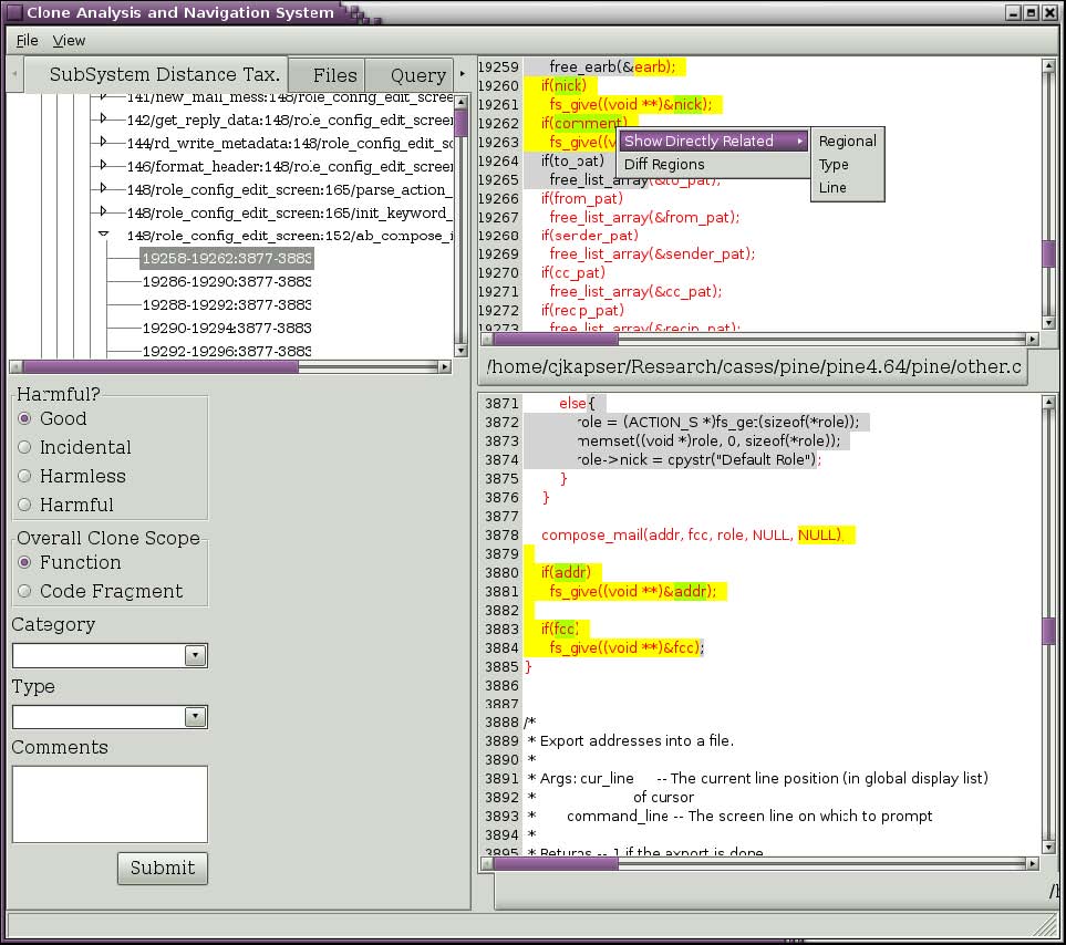
Figure 4: Query for related clones.
If you wish to see clones that are related to RGC you are currently viewing you can ask to see all clones that occur in one of the two regions. Right click on the text of interest and select one of the submenu items under the “Show Directly Related” popup menu item (seen in Figure 4). The three choices are regional, type, and line. Selecting “Regional” will return all clones that have one segment in the selected region. Selecting “Type” will return all clones that have one segment in the selected region and are of the same type you are currently viewing. Selecting “Line” will return all clones that have one segment covering the line you rightclicked on. In the past you could also make similar queries about clones using transitive closure, this feature is currently being reimplemented. Figure 5 depicts the results of selecting “Line” in Figure 4. The results, organized by the same taxonomy used in the first tab, are shown in the Query tab. This tree has the same behavior as described for our first tab.
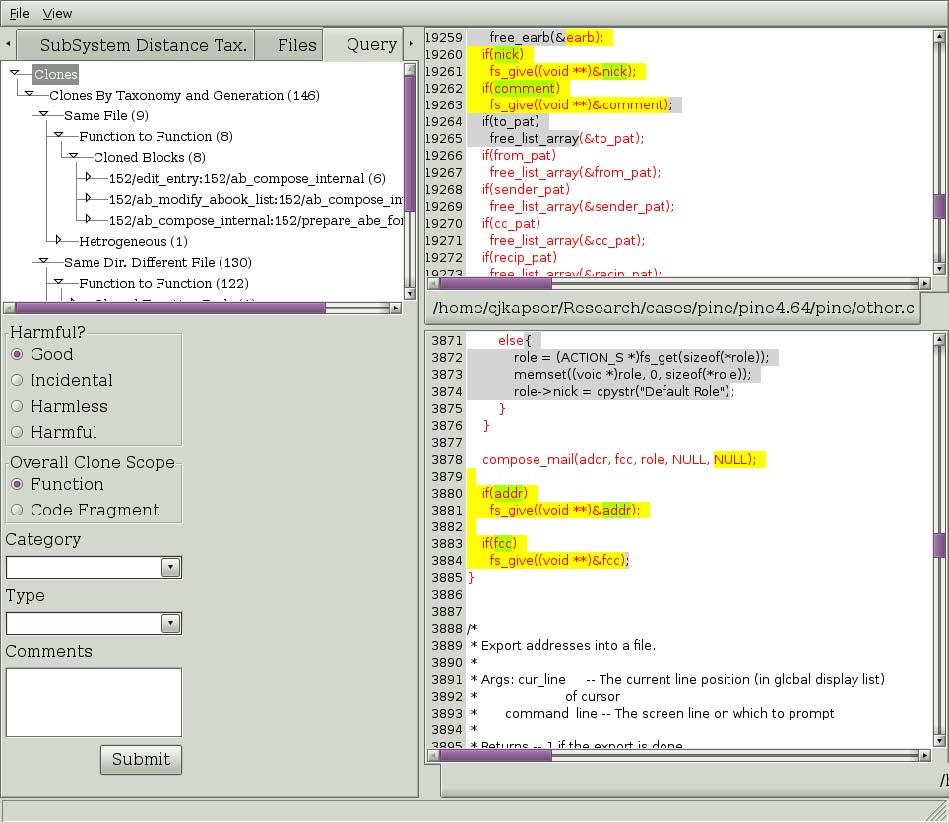
Figure 5: Result of Directly Related > Line query.
The clone detection method used by CLICS often contains false positives. These can be removed from the database as you discover them. Simply select the clone that is a false positive and then right click on it. A popup menu will appear (Figure 6). To remove all clones in the clone group, select “Remove Group of Clones”. To remove an individual clones, select “Remove Clone”. Bug: Clones are not being recategorized after removing an individual clone. To be fixed.
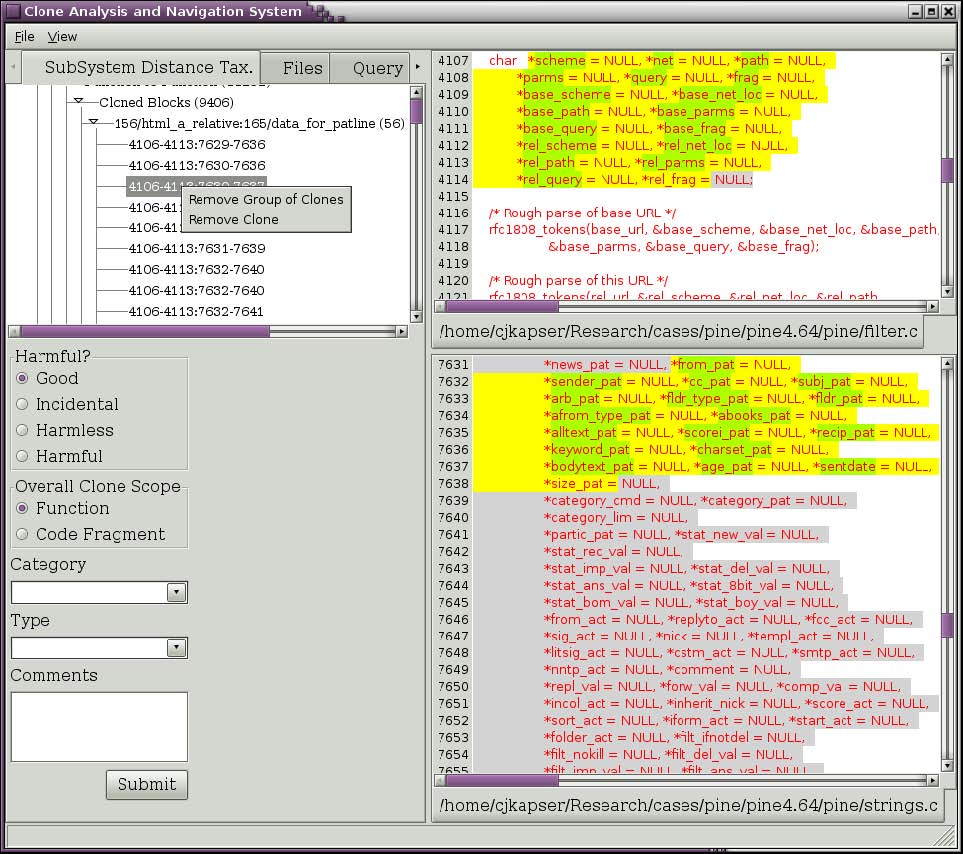
Figure 6: Menu to remove clones.
To document:
- –
- summary panel
- –
- files tab (stats grid, relationship tree)
- –
- lsedit view
References:
- (1)
- "Improved Tool Support for the Investigation of Duplication in Software", by Cory Kapser and Michael W. Godfrey. Proc. of the 2005 Intl. Conference on Software Maintenance (ICSM05), Budapest, Hungary, 2530 Sept 2005.
- (2)
- “ Cloning Considered Harmful' Considered Harmful: Patterns of Cloning in Software", Cory J. Kapser and Michael W. Godfrey. Empirical Software Engineering (Springer), vol. 13, no. 6, December 2008.